CS 7641 Final Project Report(Team 04)

Anirudh Prabakaran, Himanshu Mangla, Shaili Dalmia, Vaibhav Bhosale, Vijay Saravana Jaishanker

Proposal Link

Midterm Report Link

Introduction/Background:

“You are what you stream” - Music is often thought to be one of the best and most fun ways to get to know a person. Spotify with a net worth of over $26 Billion is reigning the music streaming industry. Machine Learning is at the core of their research and they have invested significant engineering effort to answer the ultimate question “What kind of music are you into?”

There is also an interesting correlation between music and user mood. Certain types of music can be attributed to certain moods among people. This information can be potentially exploited by ML researchers, to understand more about their users.

The use of Machine Learning to retrieve such valuable information from music has been well-explored in academia. Much of the highly cited prior work [1,2] in this area dates to over two decades ago when significant work was done through pre-processing raw audio tracks for features like timbre, rhythm and pitch among others.

The advent of machine learning has created new opportunities in music analysis through the visualizations of audio achieved through spectral transformations. This has opened the frontiers to apply the knowledge developed for image classification into this problem.

Problem Definition:

In this project, we want to compare music analysis done using the audio metadata based approach to the spectral image content based approach using multiple machine learning techniques such as logistic regression, decision trees, etc. We would be using the following tasks for our analysis:

• Genre Classification[1,2]
• Mood Prediction[3]

Genre Classification

Data Cleaning and Feature Engineering

We started with two datasets for our project - the Million Song Dataset consisting of 10,000 songs and the 1.2 GB GTZAN dataset that contains 1000 audio files spanning over 10 genres.

We used a subset of the Million Song Dataset and extracted basic features from the data that could help us in identifying the song genre like tempo, time signature, beats, key, loudness, timbre, etc. We referenced the tagtraum genre annotations for the Million Song Dataset to get target genre labels to train our models. We then removed the songs which did not have a target label, thus reducing our data to around 1.9k songs.

We did some feature engineering to calculate the means of several feature values like pitch, timbre, loudness, etc, added these analytical features values to the original dataset, and dropped all rows with NaN to create a final clean dataset.

For the spectral image content based approach, we used readily available preprocessed data converted from the raw audio to mel-spectogram using the librosa library. Each track has a total of 169 features extracted.

Exploratory Data Analysis

We set out to understand more deeply the distribution of the dataset we were using. Here are some interesting tidbits that we would like to call out.

Dataset for our metadata based approach (Million Song Subset)

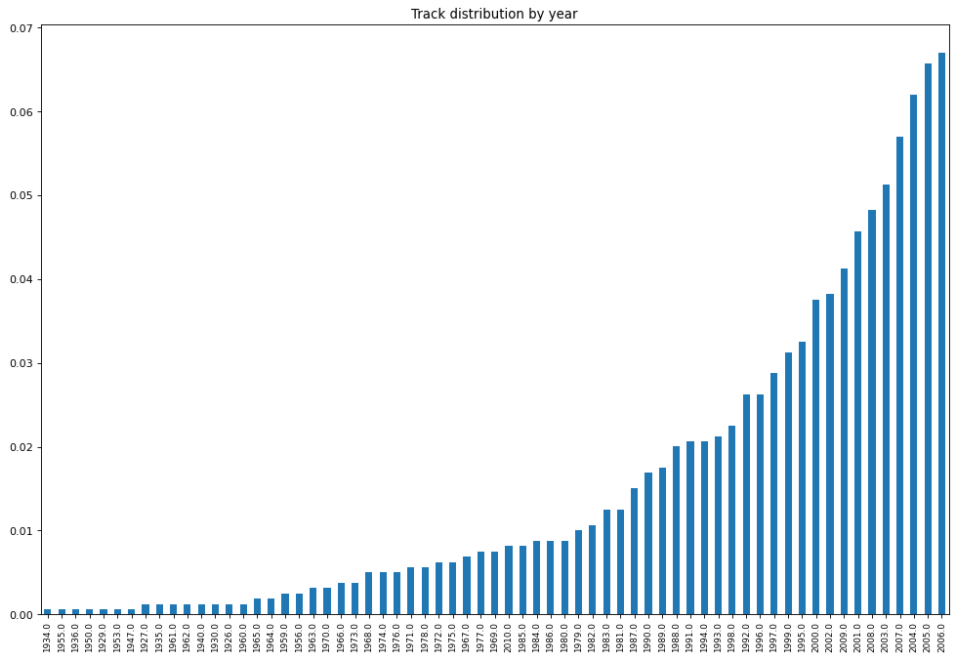
1. Most songs in our dataset were new (released after the 2000’s).

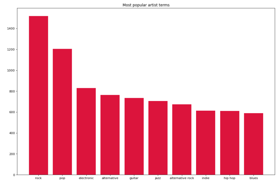
2. We saw that ‘rock’ and ‘pop’ were the most popular artist terms (tags from The Echo Nest device) used to describe the songs in our dataset.

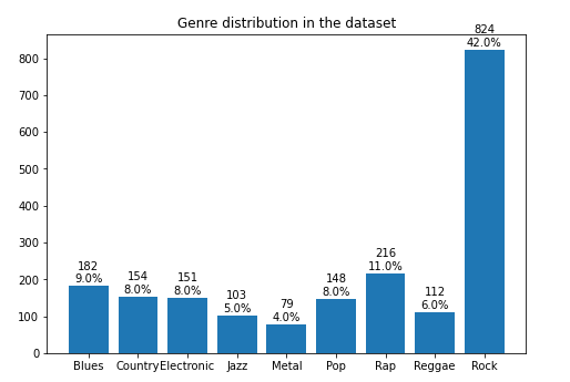
3. We analysed the distribution of genres in our dataset and found that Rock is the dominating genre with 42% of songs being rock songs. All other genres are almost equally distributed with values between 4-11%, the lowest being Metal(4%) and the highest being pop(11%).

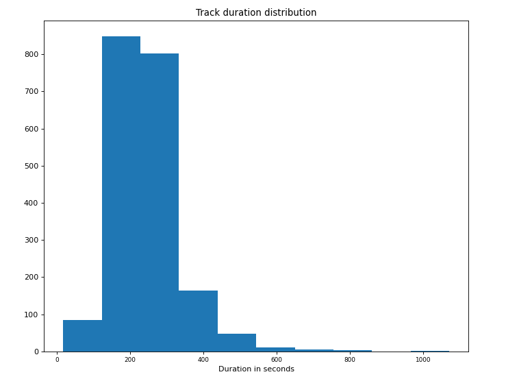
4. We analysed the song durations and found that most songs were between 150-350 seconds long.

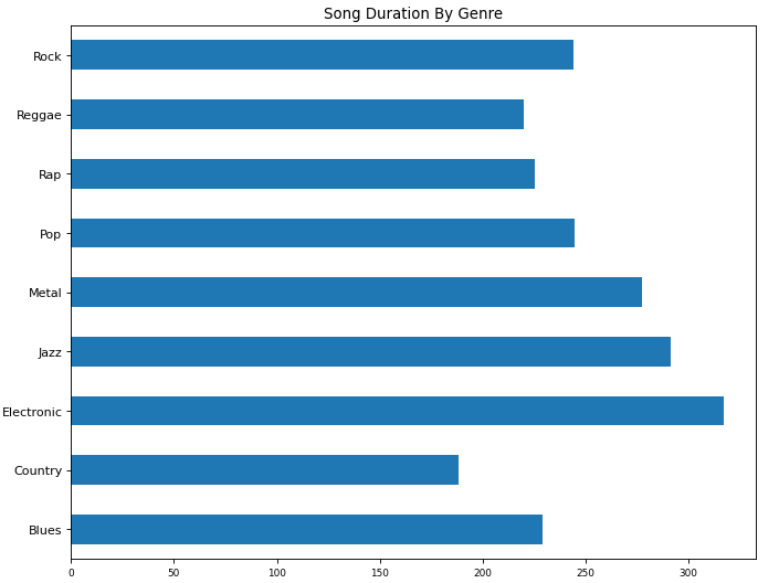
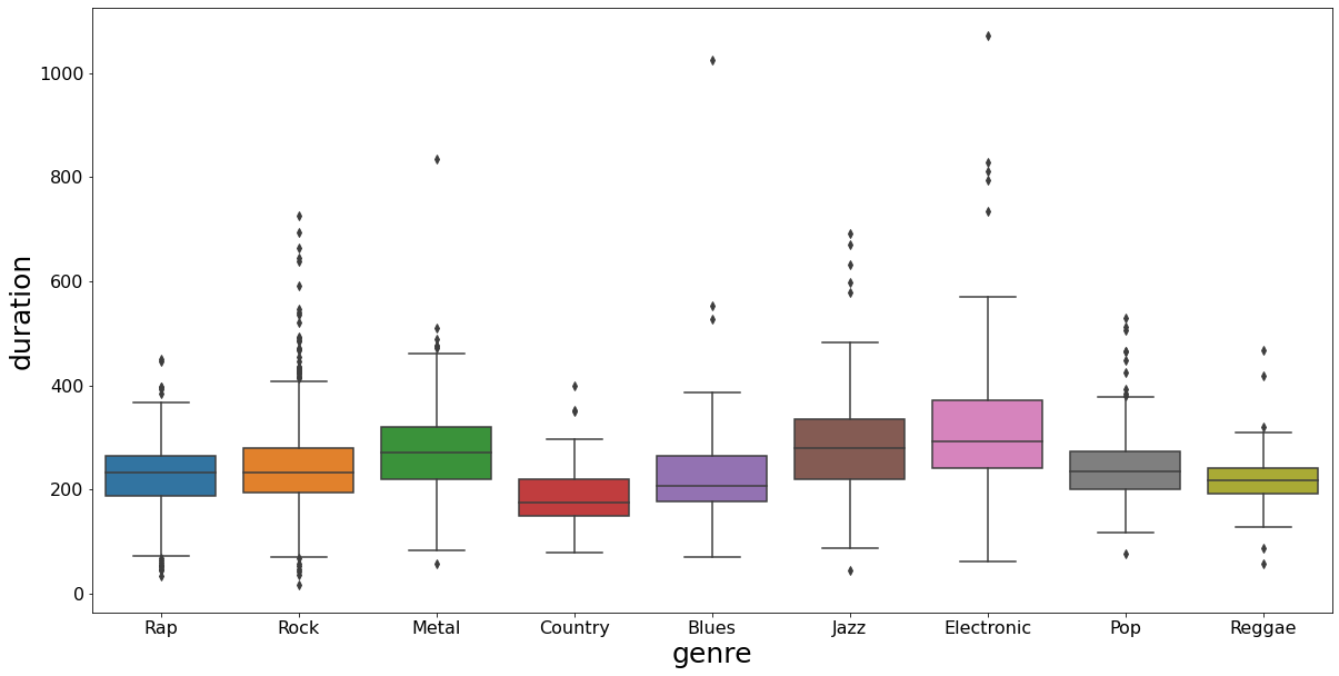
5. On organizing mean song duration by genre, we found that the electronic genre tended to have longer songs and country the lowest.

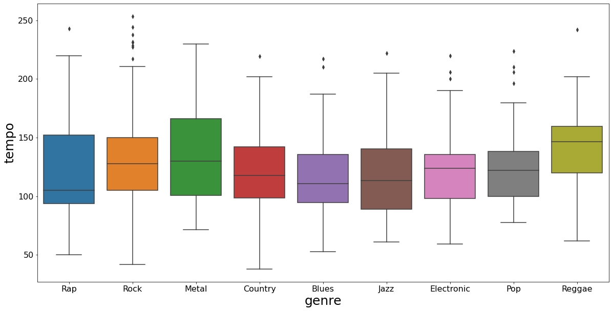
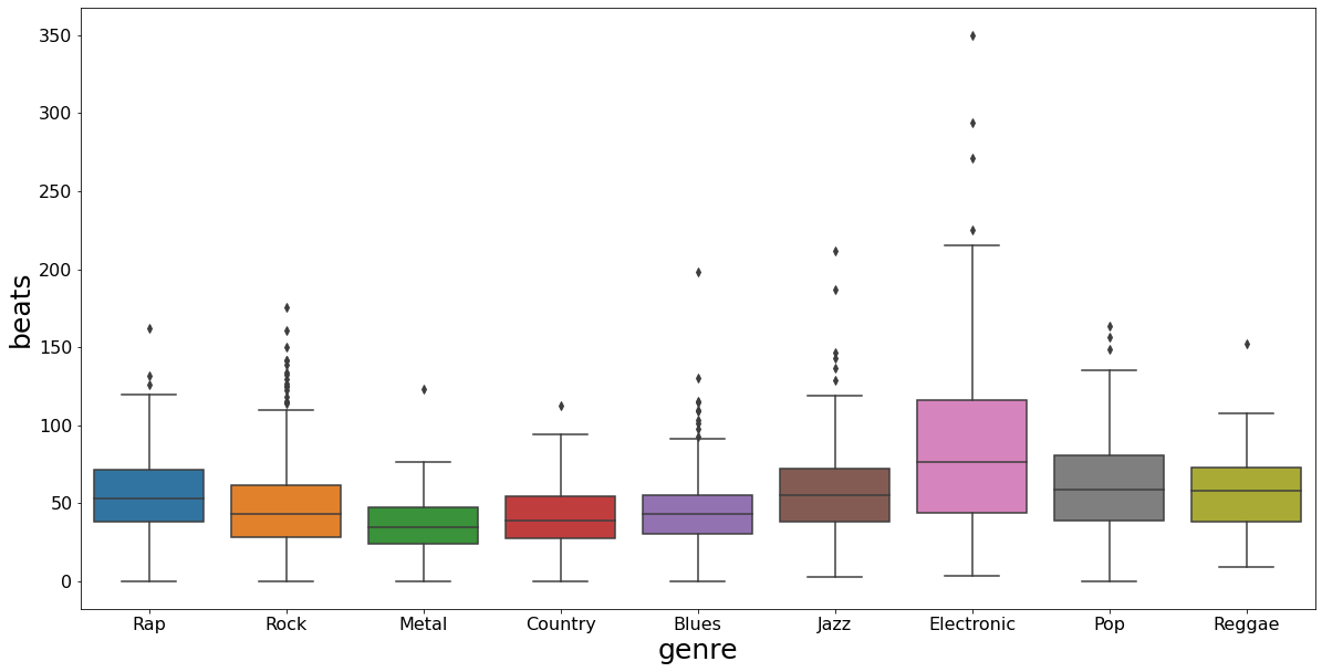
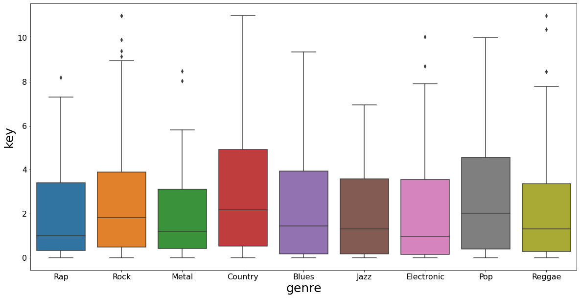
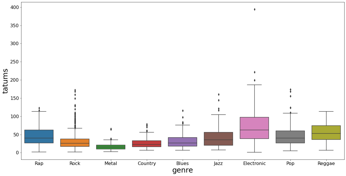
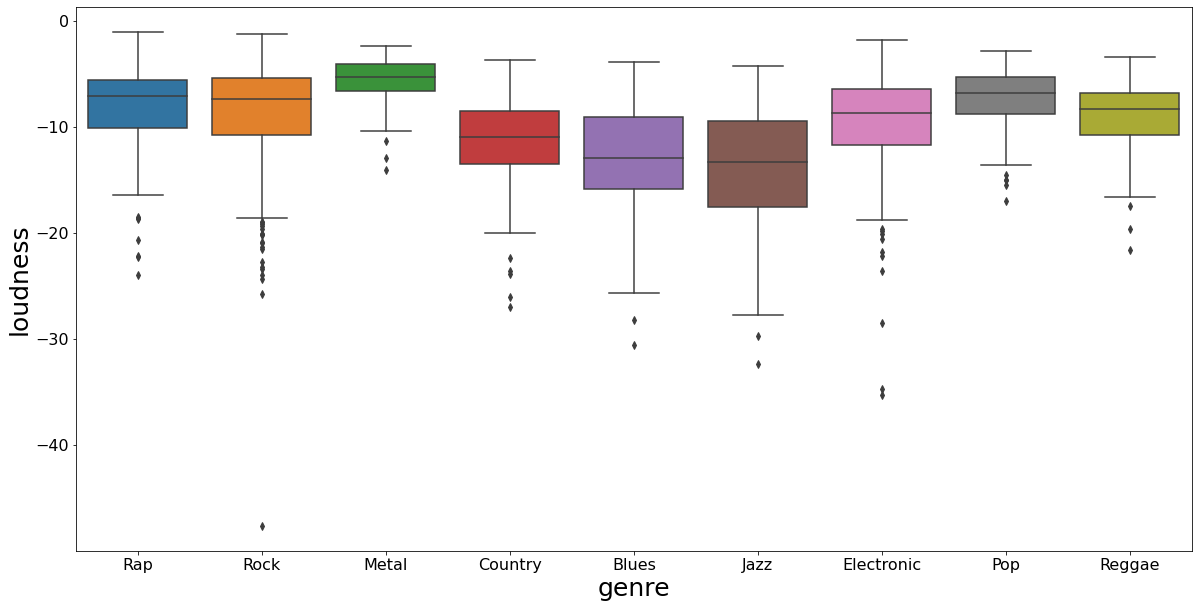
6. We wanted to analyse other features for all genres too. We noticed that Reggae has a higher mean tempo, while rap had the lowest. Pop and country were in a higher key on average than other genres. The tatum (defined as the smallest time interval between successive notes in a rhythmic phrase) was highest in Electronic. Metal was highest in terms of average loudness and as discussed before, electronic and jazz tended to have longer songs.

Dataset for our spectral imaging based approach (GTZAN)

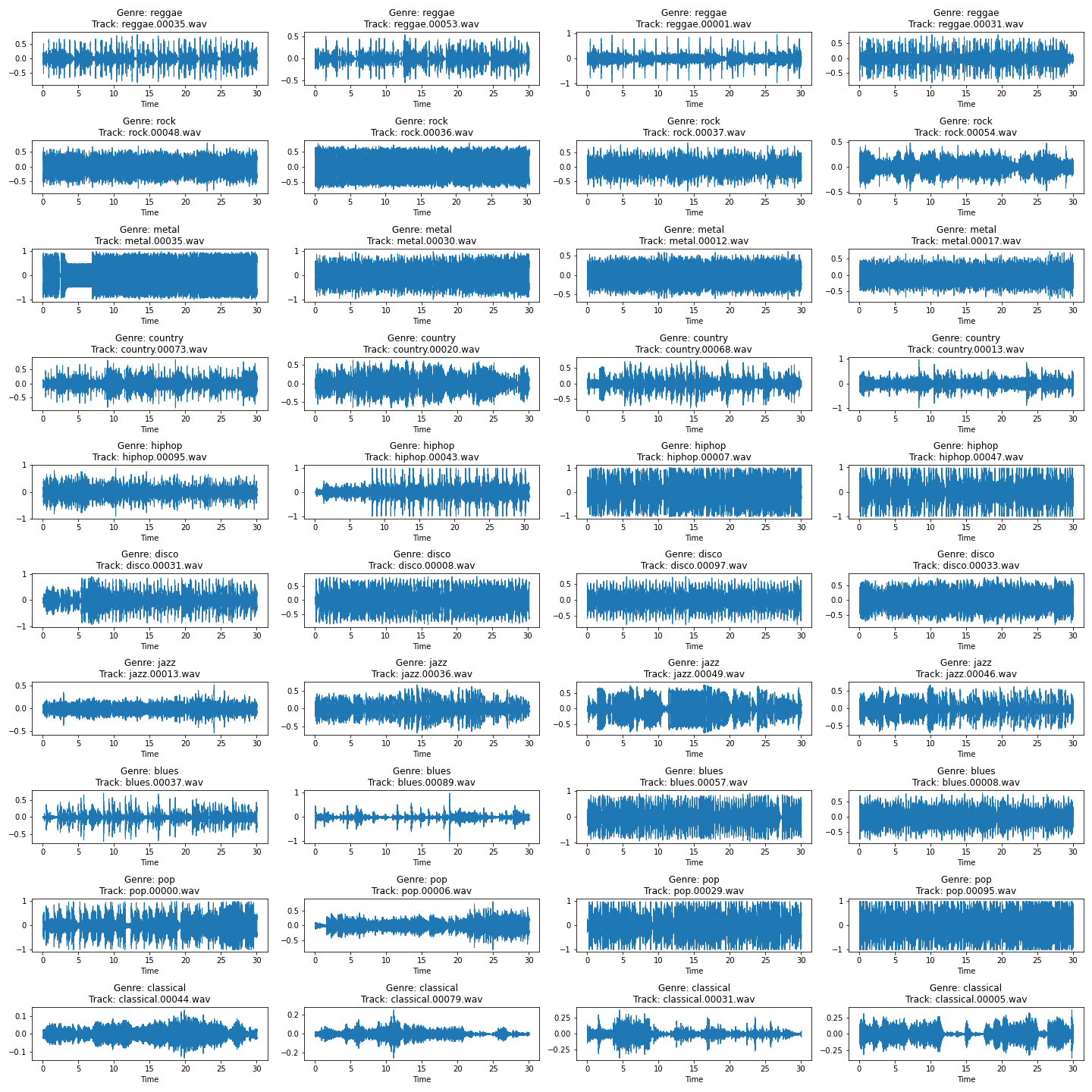
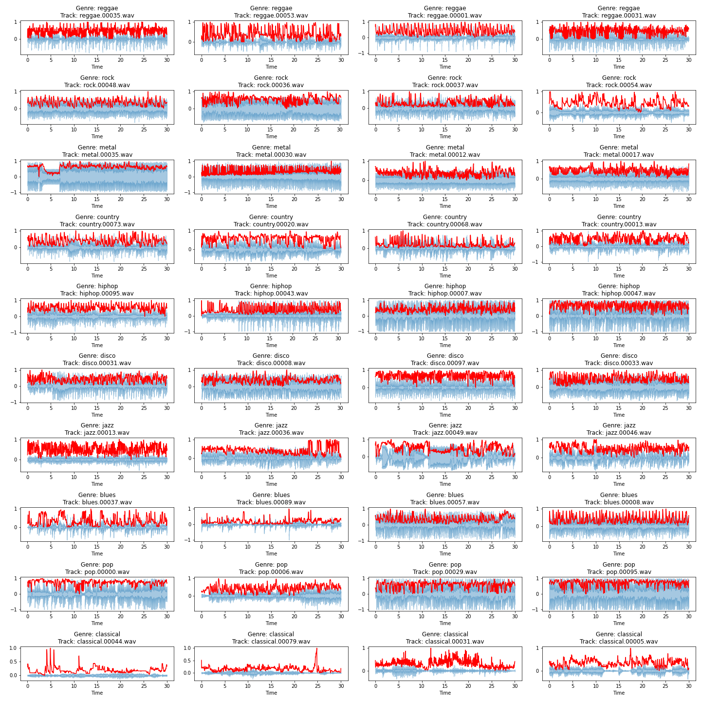
1. Time Series: We look at a time series plot to observe the changes in the amplitude. Clearly, we cannot distinguish any genre with just this data. However, we notice some information like how the variation of amplitude is very high for metal, but for genres like ‘classical’ it is pretty mellow.

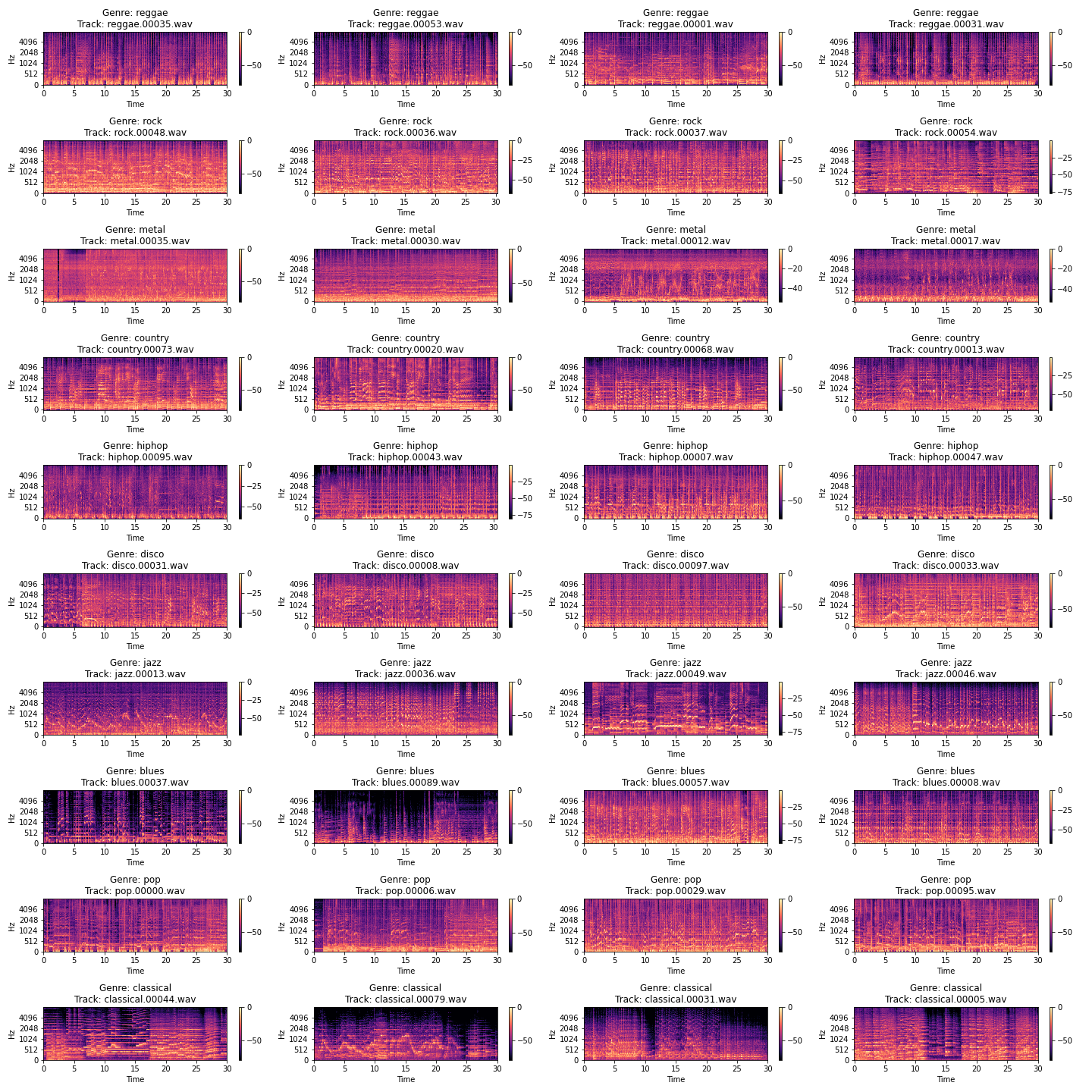
2. Spectogram: A spectrogram is a visual representation of the spectrum of frequencies of sound or other signals as they vary with time. It’s a representation of frequencies changing with respect to time for given music signals. Plotting in linear scale gives the plots as shown below. We see some interesting details like how classical songs are dominated by more high frequency sounds.

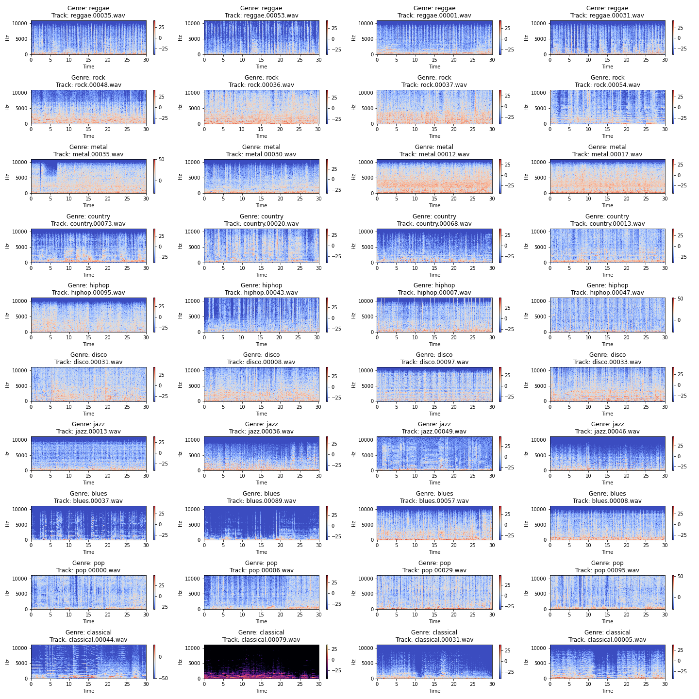
We also plot this on a log scale.

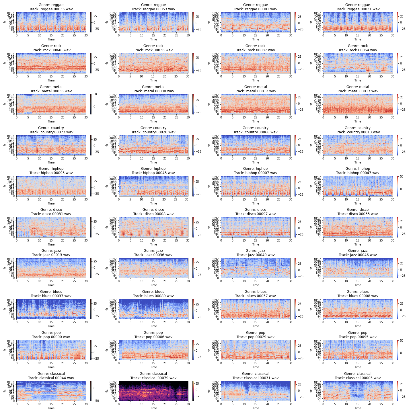
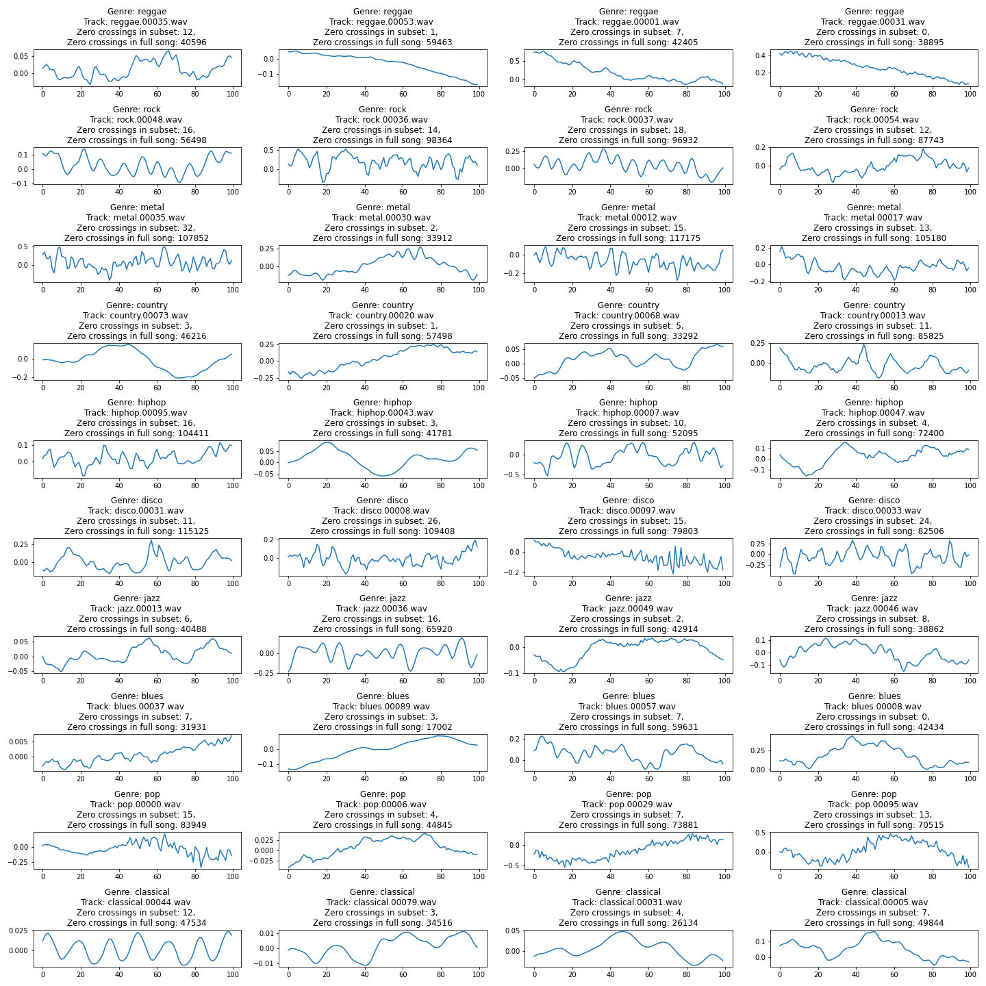
1. Zero Crossing Rates: The zero crossing rate is the rate of sign-changes along a signal, i.e., the rate at which the signal changes from positive to negative or back. This feature has been used heavily in both speech recognition and music information retrieval. It usually has higher values for highly percussive sounds like those in metal and rock. This is a zoomed in plot (small sample of the music) to show what zero crossing means. The title of each plot tells the zero crossing count for the song subset as well as for the entire song.

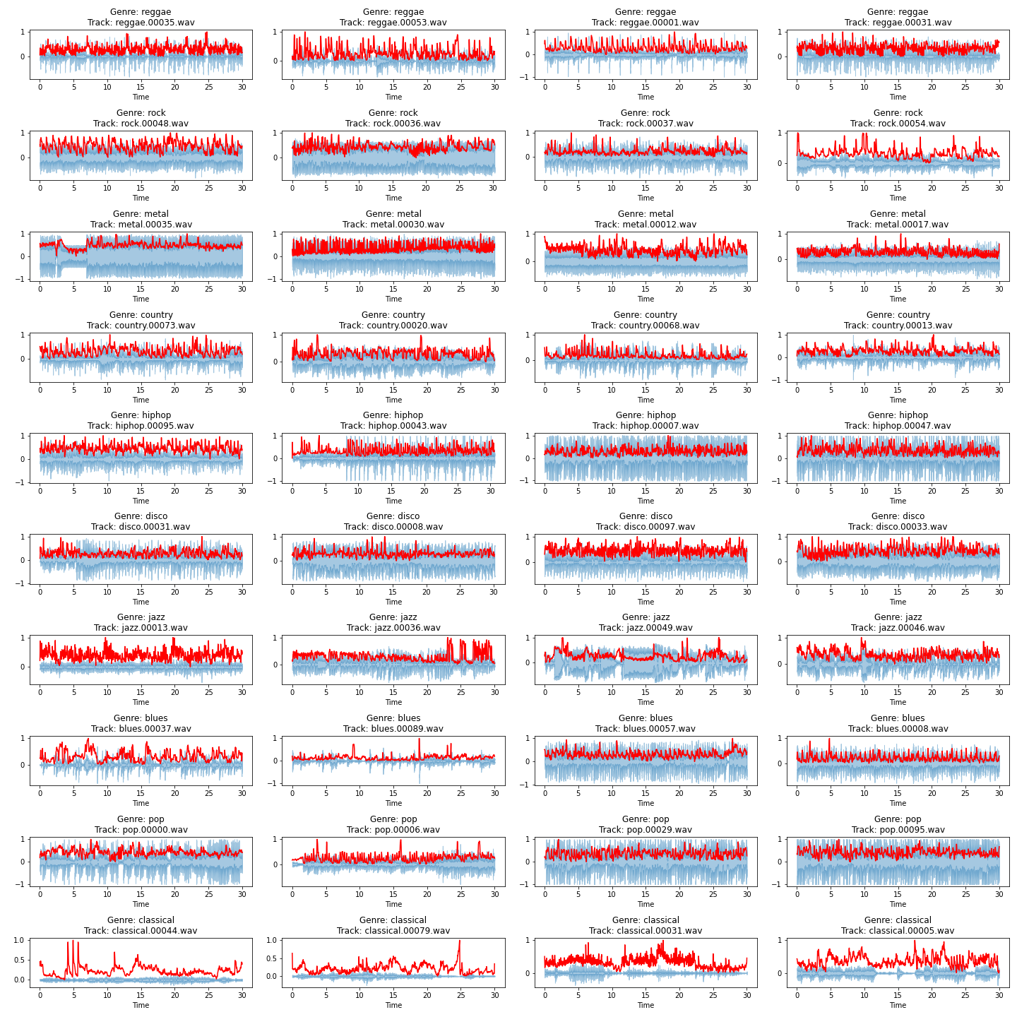
2. Spectral Centroid: It indicates where the ”centre of mass” for a sound is located and is calculated as the weighted mean of the frequencies present in the sound. If the frequencies in music are same throughout then spectral centroid would be around a centre and if there are high frequencies at the end of sound then the centroid would be towards its end.

3. Spectral Rolloff: Spectral rolloff is the frequency below which a specified percentage of the total spectral energy, e.g. 85%, lies. It also gives results for each frame.

4. Mel Spectogram

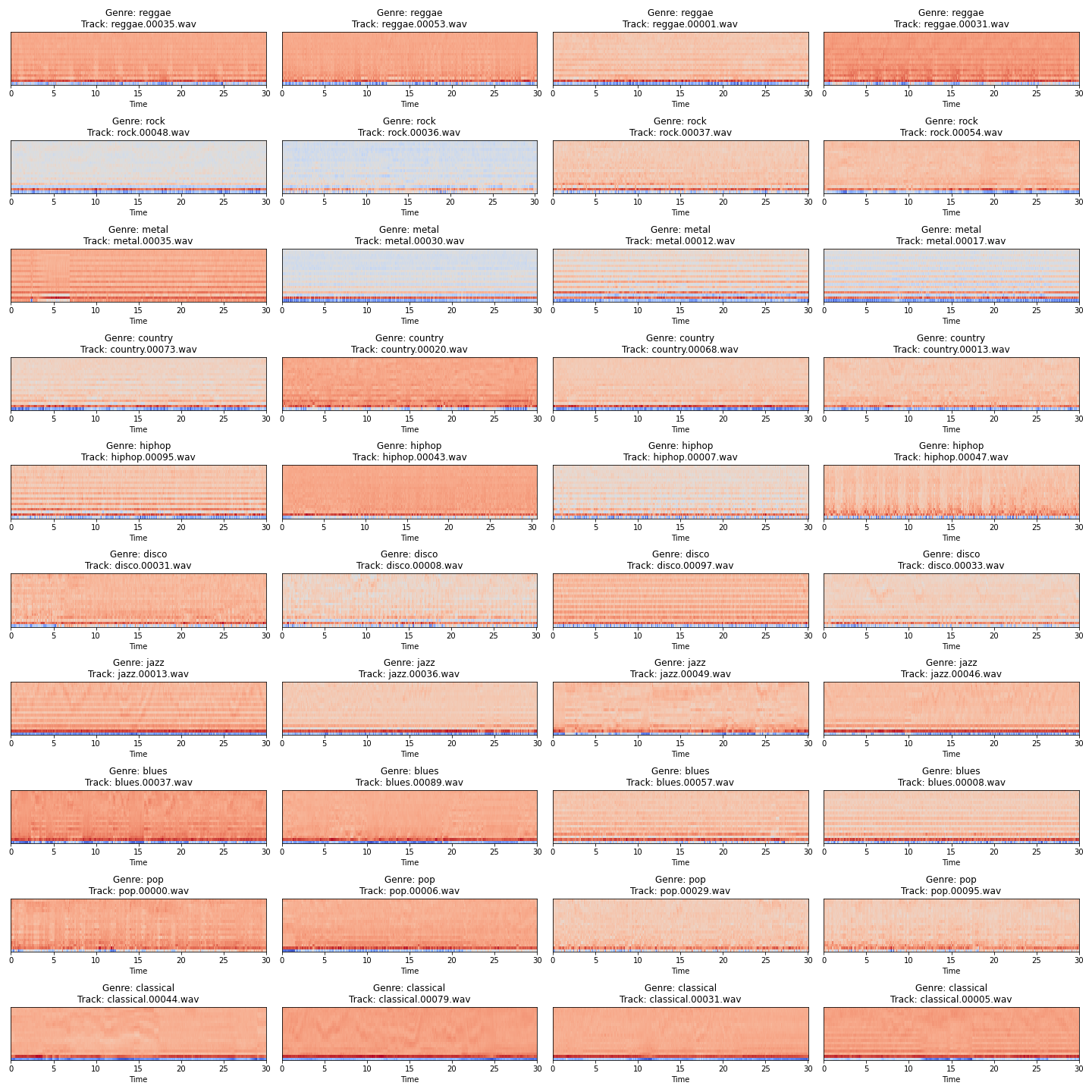
5. MFCC: This feature is one of the most important methods to extract a feature of an audio signal and is used majorly whenever working on audio signals. The mel frequency cepstral coefficients (MFCCs) of a signal are a small set of features (usually about 10–20) which concisely describe the overall shape of a spectral envelope. This is the feature we ended up choosing to train our neural net due to its ability to describe the overall spectral envelope of audio most accurately

Methods

We have tried to use both the metadata-based and spectral-imaging based approaches for genre classification.

Metadata based approach

• These models were trained using the metadata features.
• We used a 75-25 test-train split and tried the following methods.

Random Forest Classifier

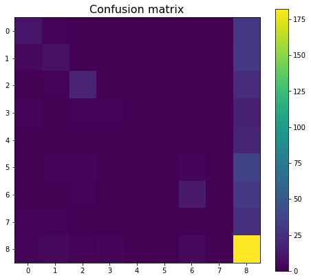
We started with a random forest classifier which provided a test accuracy of 50.7%. The confusion matrix is as follows:

Xtreme Gradient Boost(XGB) Classifier

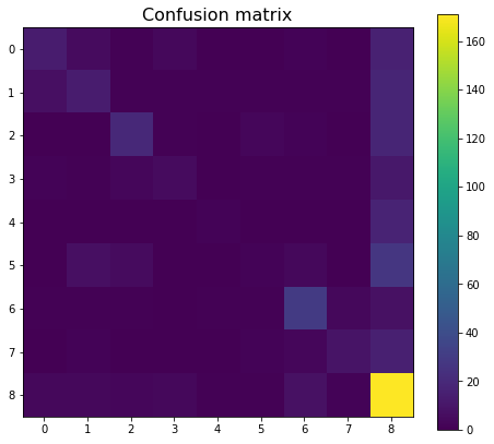
XGB classifier gave us the best results with a test accuracy of 56.1%. The confusion matrix is as follows:

Ada Boost Classifier

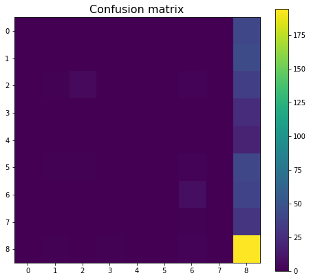
Ada Boost Classifier provided a test accuracy of 45.1%. The confusion matrix is as follows:

Logistic Regression Classifier

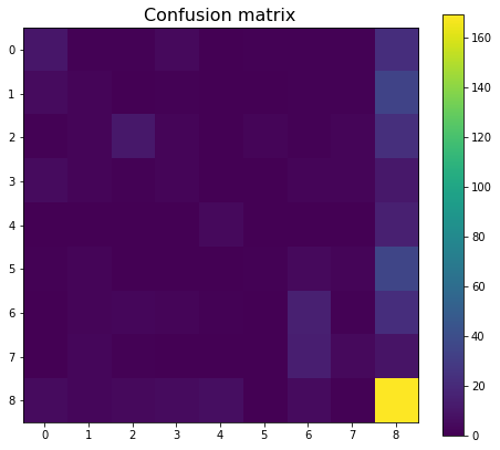
A logistic regression classifier provided the lowest test accuracy of 44.2%. The confusion matrix is as follows:

Spectral Imaging Based Approach

• These models were trained using features that we generated from raw audio.
• We used a 75-25 test-train split and tried the following methods.

Support Vector Machines

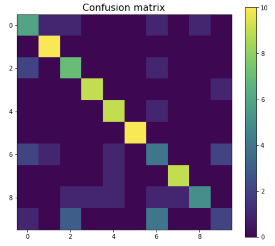
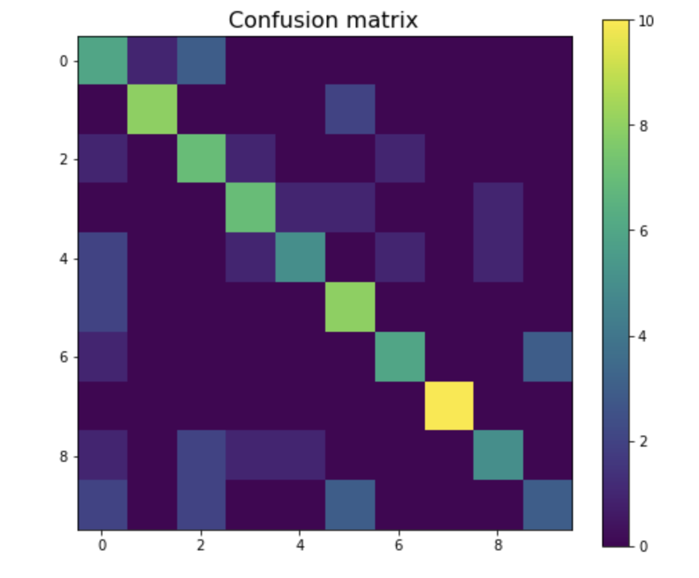
SVM Classifier provided a test accuracy of 71%. The confusion matrix is as follows:

Xtreme Gradient Boost Classifier

XGB Classifier provided a test accuracy of 65%. The confusion matrix is as follows:

Neural Network Classifier

• We define a simple sequential neural network with the following layers :

• From these layers, we computed the network by using 3 blocks of conv-relu-maxpool-dropout. The first block used a conv 2d with kernel_size=3 and 8 filters. The second block used a conv 2d with kernel_size=4 and 16 filters. The third block used a conv 2d with kernel_size=5 and 32 filters.

• Then we have 2 fully-connected layers. The last FC layer has 10 output units corresponding to our 10 genres. We use ReLU activation and a dropout p=0.1 for all layers.

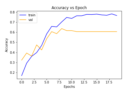
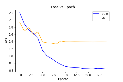
• We have used the Cross Entropy loss function and the SGD optimizer. We train the model for 20 epochs and get an accuracy score of 74.2%. The graph for epoch vs loss and epoch vs accuracy shows the increase in the model accuracy with increasing epochs and decrease in model loss with increasing epochs as expected.

Unsupervised Learning Techniques

• Over the GTZAN dataset of 10 genres, we drop their labels and extract a vector representation for each of the data tuples. We obtain a 169 dimensional feature space for them using librosa.

• Over these features, we try to perform unsupervised learning to see if similar files are placed together in the same clusters. We employ K-means and Hierarchical Agglomerative clustering over them.

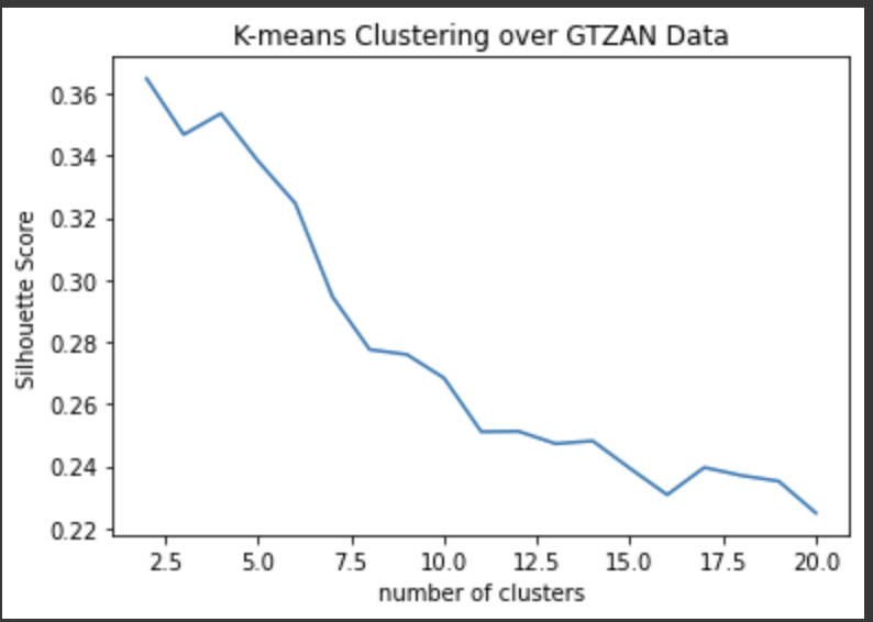
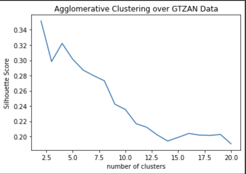
• Since an unsupervised learning technique cannot be directly evaluated due to unavailability of ground truth, there are certain internal metrics which can measure the performance of clustering algorithms. Once such metric is called Silhouette Coefficient. It is a ratio of the inter cluster distance with the intra cluster distance. It is a bounded value between (-1, 1). This dictates that if two points in a cluster are closer, the silhouette coefficient will be higher and similarly if two points in different clusters are farther, the silhouette coefficient will be higher. A negative value for this implies poor clustering performance.

• While K-means is a fast algorithm, it is highly dependent on the initialization of cluster centroids and the ‘number of clusters’ parameter. In our experiment over the 1000 tuple data, we vary the number of clusters from 2 to 20 and see that we are able to obtain a silhouette coefficient of 0.27 with 10 clusters. Such a performance could be due to two reasons:

  • Lack of enough training data: We only have a 1000 tuples which may not be sufficient for training a good enough model
  • High Dimensional Data: Our dataset comprises 169-dimensional input vectors. Such high dimensional data can be hard to understand and developing an effective clustering model can be a challenging task.

• We also performed an experiment with Hierarchical Clustering. While it is computationally expensive to perform, it often is useful when data samples are smaller in size. Here too, we perform an experiment with ‘number of clusters’ varying from 2 to 20 and are able to obtain a Silhouette score of 0.23 over 10 clusters.

Results

• We summarize the different metrics for all the approaches we have used below for genre classification

Metadata Based

• We obtained the following test results:

Index	Model	Score	Top2 Accuracy	Top3 Accuracy	Top5 Accuracy	Precision	Recall	F1 Score
0	XGB	0.561653	0.705882	0.807302	0.916836	0.450703	0.355686	0.376163
1	Random Forest	0.507446	0.669371	0.776876	0.910751	0.312911	0.235179	0.243153
2	ADA	0.451220	0.606491	0.734280	0.894523	0.194109	0.138401	0.112782
3	Logistic Regression	0.442191	0.624746	0.740365	0.898580	0.320230	0.240084	0.249590

Spectral Imaging-Based

• We obtained the following results:

Index	Model	Score	Top2 Accuracy	Top3 Accuracy	Top5 Accuracy	Precision	Recall	F1 Score
0	SVM	0.71	0.88	0.93	0.97	0.7079	0.71	0.69903
1	XGB	0.65	0.84	0.9	0.98	0.67389	0.65	0.649
2	Neural Network	0.7425	0.9207	0.9405	0.99	0.7269	0.7371	0.7186

Mood Classification

• The mood of a song is not very straightforward to compute. A song can sound very happy, however the lyrics can be extremely negative. An example would be ‘Pumped Up Kicks’ by Foster The People, which has a mellow and a chill beat but the lyrics reveal an intention for revenge. So, getting labelled data was very hard as most of the data was not trustworthy and involved arbitrary labelling of the songs.

Dataset

• We used the MUSE dataset (The Musical Sentiment Dataset) which has a collection of 90001 songs with all relevant mood annotations. The process used by the authors to curate the dataset is summarised below.

  • Get 279 mood labels from AllMusic.
  • For each label, query lastfm to collect 1000 songs for each mood. They ended up with 96499 songs.
  • Filtering is performed to take songs with at least one mood.
  • Mapping of the moods to the Russell’s (1980) “circumplex model” is performed. Get the corresponding V-A-D (valence, arousal, dominance) tags for each song.
  • Append spotifyURI, musicbrainzID to the song.

• Using the dataset as a seed, we expand it further by querying the spotify API with the spotify URI of each song to extend the dataset. Moreover, we focus on the most important 4 moods - ‘happy’, ‘angry’, ‘sad’ and ‘calm’. Which leaves us with 2633 songs in total.

Exploring the Data

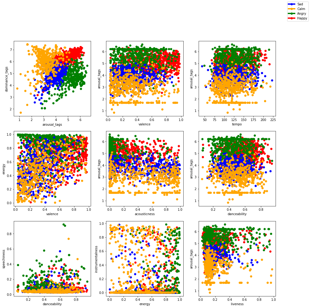
• We start with cleaning the obtained data by solving class imbalance - maintaining about 500 songs per class. We create a dataframe by dropping unnecessary columns and try plotting correlation between features. Out of all the features, we find the following correlations intuitive.

• By plotting this, we can see the importance of features such as dominance, arousal, valence, energy etc. In most of the graphs, we can see that the moods sad and calm lie closer and happy and angry lie closer to one another. This is expected because of the valence, energy components of the sad/calm songs are similar and likewise for happy and angry songs.

• We further plot the importance of various features for various moods using a radar chart and we find the following results.

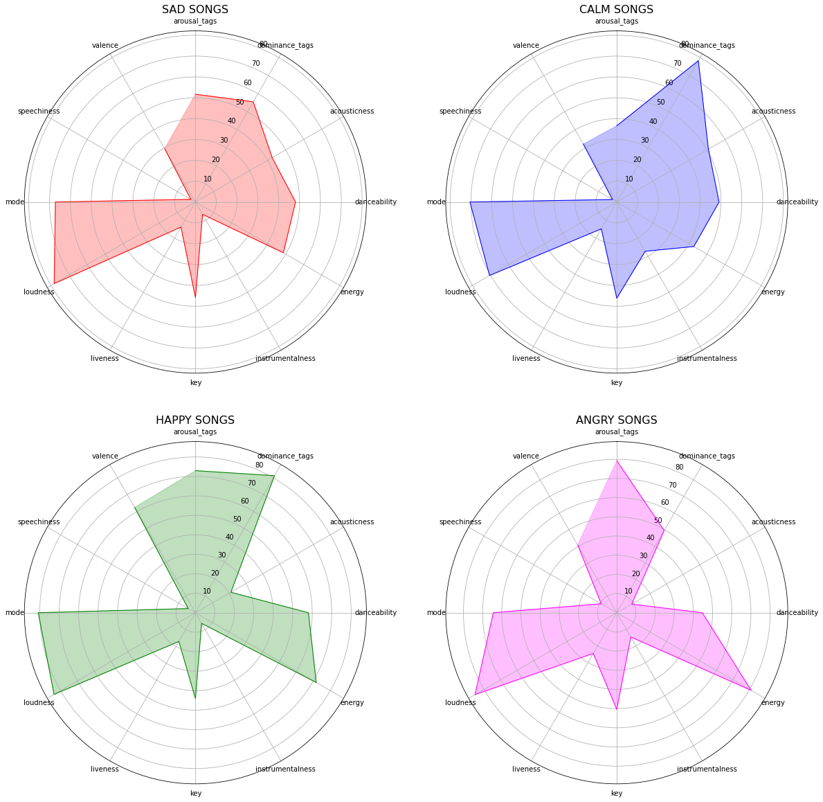
• We can see that the energy, arousal and valence components of happy and angry songs are similar (high) and low for sad and calm songs. We also see that sad and calm songs have more acoustic-ness. We can also see some difference between sad/calm and angry/happy songs as well which would help in the classification later.

Fitting Models

• Before fitting the data to our models, we do a train test split with a test size of 20% which we will use for all our chosen models.

Random Forest

• We start with the random forest classifier which provides us a test accuracy of **0.85%. **The confusion matrix for the random forest classifier is as follows :

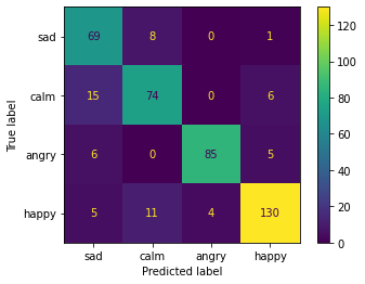
• The good performance of the random forest classifier could be attributed to the fairly low number of features (13 features).

SVM

• Fitting the SVM classifier yields fairly good results - giving about 87% test accuracy. The confusion matrix is as follows.

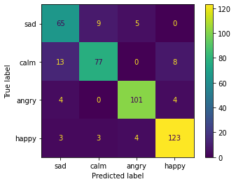
• This good performance can be due to the fact that the data could be linearly separable by projecting in higher dimensions. From the correlation plots, we can see that some features separate the data points well based on the mood in the 2D plane.

K Means

• Though we are working on labelled data, we tried fitting a K Means model on the data to look for the number of clusters based on the elbow method. We plot the distortion based on the number of clusters and as seen below we can see the elbow at number of clusters = 4.

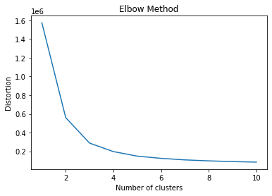
• We later try to calculate the accuracy of the K Means model on the dataset by calculating the number of correctly classified data points. Since, the number of classes is 4 - the K means does a poor job in the classification problem with an accuracy of 0.10. Only 176 out of 1674 samples were labelled correctly. This is expected because, even if K means rightly separates the data into clusters - it could misclassify class ‘sad’ as class ‘calm’ and so on due to the unsupervised method.

KNN

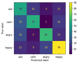
• KNN performs the worst out of all the models giving an accuracy of 62% on test data. The confusion matrix is as follows for number of neighbours = 5:

• We also tried varying the number of neighbours and found that the accuracy decreases as we increase the number of neighbours, giving maximum accuracy with number of neighbours as 1 :

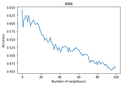
• Poor performance of KNN could be due to the problem of the curse of dimensionality and randomness of the data. KNN is suitable for data which is well separated and defined and does not have a lot of features. We could see from the correlation plots that a lot of data points were very close to each other in the 2D plane. And this could lead to a lot of misclassification for our KNN model causing poor performance.

Neural Network

• We define a simple sequential neural network with the following layers :

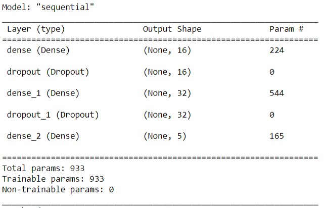
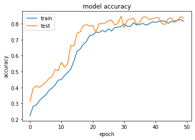
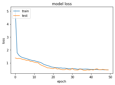
• We have used the loss function ‘categorical_crossentropy’ and adam optimizer. We train the model for 50 epochs and get an accuracy score of 84%. The graph for epoch vs loss and epoch vs accuracy shows the increase in the model accuracy with increasing epochs and decrease in model loss with increasing epochs as expected.

Results

• We summarize the different metrics for all the approaches we have used below for mood classification

Metadata Based

• We obtained the following test results:

Index	Model	Score	Top2 Accuracy	Top3 Accuracy	Precision	Recall	F1 Score
0	Random Forest	0.832935	0.976133	0.99761	0.839638	0.832935	0.834883
1	SVM	0.863961	0.973747	0.995226	0.867356	0.863961	0.865655
2	KNN	0.551312	0.773269	0.902147	0.562860	0.551312	0.557026

Conclusion

As we had expected, we ended up spending significant amount of time in data engineering. Our results for genre classification validated our hypothesis that the spectral imaging based approach seems to be performing better than the metadata approach since it is able to take into account features that form the audio composition of the song, which is in sync with how humans have performed genre classification so far.

Machine Learning in music is a hot area of research. Companies have invested millions to try and understand music and user preferences. Through this project we had the opportunity to experiment with various types of models that we learnt in class. Additionally, we learnt a great deal about audio processing and various components that distinguish each track of music that we hear on a daily basis. It was interesting to plot our various findings and correlate it to our general music knowledge. Tag prediction, Music recommendation systems are other related interesting problem statements that we hope to take up in the future.

References

[1] Tzanetakis, G., & Cook, P. (2002). Musical genre classification of audio signals. IEEE Transactions on speech and audio processing, 10(5), 293-302.
[2] Scaringella, N., Zoia, G., & Mlynek, D. (2006). Automatic genre classification of music content: a survey. IEEE Signal Processing Magazine, 23(2), 133-141.
[3] Delbouys, R., Hennequin, R., Piccoli, F., Royo-Letelier, J., & Moussallam, M. (2018). Music mood detection based on audio and lyrics with deep neural net. arXiv preprint arXiv:1809.07276.
[4] Kaggle Million Song Dataset : https://www.kaggle.com/c/msdchallenge
[5] Music Genre Classification | GTZAN Dataset : https://www.kaggle.com/andradaolteanu/gtzan-dataset-music-genre-classification